
|
| Elliott Sound Products | PSU Simulation |
 Main IndexArticles Index
 On the surface, simulating a power supply (regardless of the simulator you use) is simple. A sinewave generator producing the nominal mains voltage and frequency, perhaps an 'ideal' transformer with the correct ratio(s), some diodes and filter capacitors. Then you apply a load to see the ripple performance, and perhaps examine regulation, filter capacitor ripple current and diode dissipation. The load can be varied so you can observe the performance with different output current.
It all seems very straightforward, but there are so many traps and 'gotchas' hiding within this simple model that you will almost certainly be bitterly disappointed when the 'real thing' (i.e. the finished physical power supply) doesn't behave even remotely like the simulated version. The reasons are often puzzling, but there are many things you need to do to get a reasonably accurate simulation working.
There are many reasons to simulate power supplies, not the least of which is that you can do anything you like. Short circuits or insanely low load impedances won't harm the simulator one bit, where a physical supply may be destroyed by the same abuse. This is one of the beauties of simulations - you can try anything, however outrageous, without risking damage to hardware or yourself. Bench testing means that you have to get things right, or 'bad things' are likely to happen (such 'bad things' can also be rather expensive).
I suggest that you read the Transformer articles (there are three in the series) to ensure that you have a full understanding of the principles of transformers before you try any serious simulations. There are many factors to consider, but I will only cover the essentials here. While there are some liberties taken in this article, you will get simulations that are closer to reality than you can ever get if you don't take the most important factors into account.
Some may well ask why anyone would bother simulating such a simple circuit that's easy to put together on the bench. There are many reasons, with the most important being understanding what goes on. A simulator lets you do anything you like, and it also lets you measure things that are very difficult in a real power supply. You can use a huge filter capacitor, and none of it costs a cent - no parts to buy, no soldering, and an opportunity to examine aspects of performance that can't be done with the physical supply. Even something as simple as measuring capacitor ripple current will upset a real circuit due to the resistance of the test leads and the internal resistance of the ammeter. In a simulation, it's as easy as probing a wire for voltage or current.
Simulators often allow the use of 'ideal' parts, which you can mess with by adding series or parallel resistors, or specifying the part's parameters. This lets you see the changes quickly, and with a resolution that is usually impossible with normal test equipment. In so doing, you can use it as a learning exercise. A great many ESP articles use simulations, because it lets me produce graphs and measurements that would be very difficult and time-consuming otherwise.
Note Carefully: There is one major difference between simulating a power supply and the 'real thing'. In a simulation, it's usually not possible to account for saturation. While this might seem to be a serious limitation, it's not (although it lack of saturation does increase primary current settling time if the voltage is applied starting at 0V). Any transformer has the maximum flux density in the core at no load, and as the loading is increased, flux density decreases. This may be counter-intuitive, but it's a fact nonetheless, so any transformer simulation you perform is only very slightly affected by the inability to simulate core saturation. For the most part it can be ignored, because saturation is (almost) irrelevant at reasonable power levels.
While this article shows a step-down transformer for the examples, step-up transformers - as will be used with valve (vacuum tube) gear - can be simulated just as easily. The HV secondary winding will have a fairly high resistance, so it's easy to measure a few samples with an ohmmeter, and the forward resistance of valve rectifiers (which IMO can't be recommended for anything other than the bin) is easily simulated by adding the value shown in the datasheet for forward resistance (which may need Ohm's law to determine). Depending on the rectifier valve, expect somewhere between 50Ω to 100Ω for each diode. Otherwise, there are no surprises, other than the inevitable surprise you get when you realise just how accurate a simulation can be, once everything is included. Even choke input filters can be simulated if you wanted to go that far, and the results will be as good as your input data.
Many people use LTspice for simulations, and there are a few tricks that are necessary to 'create' a transformer. Firstly, you need to create two inductors (one for primary, one for secondary) with the inductance ratio set for the turns ratio. For the examples used below, you'd start with the primary inductance (L1) at (say) 10H, and the secondary inductance (L2) at 100mH (10:1 ratio). Note that the inductance ratio is the square of the turns ratio! Then you must add a spice 'directive', such as 'K1 L1 L2 1' to tell the simulator that the two inductances are coupled with a coupling factor of unity. If preferred, you can use a figure just below unity (e.g. 0.9999), but that's rarely needed and makes little difference. The series resistance of each inductor can be included when it's created, but it's better to keep this external so it can be seen readily (and appropriately annotated). Annoyingly, LTspice complains if you tell it that the transformer is T1 - the letter 'T' is reserved for a transmission line. Creating a simple switch is a bit of a task in LTspice, so you'll need to look at the circuits below (Figure 1).
While LTspice does have a component called a 'switch', it isn't defined, and a 'bespoke' definition has to be created for it. Nothing particularly difficult if you're familiar with the process, but more work than it should be.
If you use SIMetrix, you simply add an 'ideal transformer', with the ratio set for the desired value(s) between primary and secondary. The coupling factor can be reduced from the default of unity, but again, it's not necessary. You only have to specify the primary inductance, and the secondary looks after itself. Overall, I find SIMetrix far easier to use than LTspice, but the free version does come with limitations. A simple switch is easily created, and you just need a DC (single pulse) supply delayed by 5ms (50Hz) or 4.6667ms (60Hz).
In either SIMetrix or LTspice, the switch is driven from a single pulse source, with a voltage of between 5-12V, and the output delayed by the required time for ¼ cycle so the mains is switched on at the peak of the waveform (see the reasons for this below). The pulse duration (period where the output is at 5-12V) must be set for longer than your simulation run-time. Around 10 seconds is usually more than enough, but you can make it longer if preferred.
While there are many other versions of Spice available, I can't comment on how to use them all for the simulations shown below. If you use something other than SIMetrix or LTspice, you'll probably also know how to create the various parts as described above in the Spice version you use. If not, or if you don't use a simulator, then I suggest SIMetrix. IMO it's far easier to use than LTspice, although it does have limitations in the free version. LTspice is free and virtually unlimited, but somewhat predictably the parts offered are those made by Linear Technology (although other libraries are available).
While there are web-based simulators available, this isn't an approach I'd take. If the load is high (many users at the same time) your simulation may be queued, or if the queue is full, it won't run at all. A 'desktop' application is always preferable, and you can have as many simulations as you like, all stored on your hard drive and ready to go. For example, I have over 5,600 different simulations, saved over many years. I can load and run any of them with a few mouse-clicks, and in many cases a 'new' simulation is built from something pre-existing, with a few modifications as required.
Figure 1A, 1B - LTspice (Top) and SIMetrix (Bottom) Simulation Circuit
The two circuits shown above are screen captures, and they are functionally identical. The LTspice drawing is larger only because that's how it turned out when I took the screen grab. The remainder of the circuitry described below is simple to include in either version of spice, and changing the series resistance and other parameters are equally straightforward. The switch simply enables you to measure the primary current without the DC offset, and without having to run the simulation for longer than necessary. I would still advise that you use around 250ms for the simulation, with data output starting from the 150ms point. All circuits take some time to settle, and delaying the output trace means that you see the 'steady state' conditions.
Note that the 'pulse' directive is identical for both versions. The first number is the start voltage, followed by the output voltage, time delay, risetime, fall time and duration. The way the two versions covered here operate are very similar (probably close to identical), but the schematic capture and probe functions are quite different. SIMetrix has (IMO) a better user interface, and better (simpler) control of the graphical output. However, moving from one to the other isn't easy, as both have idiosyncrasies that take time to learn.
Figure 1C - SIMetrix Alternate Switch Circuit
The drawing above shows how you can implement a switch in any simulator, including those that don't have this functionality. The circuit shown is a MOSFET relay, and you can use any available MOSFET that has the voltage rating needed, as well as a low RDS (on). Note that the pulse generator is set for an output voltage of 10V, to ensure the MOSFETs conduct fully. The IRFP240 (20A, 200V, 140mΩ RDS-on MOSFET is a good choice, but any other MOSFET with similar ratings will work just fine. This shows one of the nice things about simulators - you can do things in a simulation that would be very tiresome in a real circuit. This can be a shortcut, or to achieve an end goal that would otherwise be hard to realise due to simulator limitations. For what it's worth, I can tell the reader from firsthand experience that setting up a physical peak switching circuit is not simple, even though it appears so in a simulator! I built one several years ago (and results are shown in the transformer articles), and it was anything but a simple circuit when completed. It can switch at either the zero crossing or peak of the waveform, but it never made it as a project because it's a 'single purpose' test tool that few people will ever need.
You don't have to include the peak voltage switch unless you intend to examine the primary current. Personally, I think it's both important and educational to do so, but for a quick simulation it's not essential. Leaving it out means there's less faffing around, and the secondary will perform normally (transformers don't pass DC, so the offset is immaterial). However, it's worthwhile to include the delayed switch so you can measure the primary current. I suggest you try it both without and with the switch, so you get an appreciation for the way inductive components react when driven from a voltage starting at zero vs. the voltage starting at the peak.
Also, be aware that peak switching causes the first half-cycle current to be very high. In the simulations shown here, it will be close to 20A, but being a simulation that doesn't matter. if you wish to measure the RMS current, you need to exclude the first 20ms of the simulation or the result will be wrong. Most simulators let you start the output trace at a specific time from the start of the analysis.
As already suggested, one of the aims of simulations it to learn how components behave, and simulation is not just a 'short-cut' design process. While it also serves that purpose admirably, you can gather so much more information from your simulated circuits, with zero risk. Simulators are powerful tools, and when used wisely can provide you with a great deal of knowledge and understanding of circuit behaviour than just building the circuit and using it. Do you trust the simulation implicitly? No. It can only be trusted if you include all of the 'real world' parasitic components, something that's close to impossible. In reality, even that doesn't mean your circuit will work as expected, and only experience will tell you if the simulation is 'sensible' or not. A simulator has no difficulty at all with telling you about circuit performance at -200dB or at a voltage of 1GV (1,000MV), but of course this is meaningless with any real circuit. However, there is so much more to them that not using one means that you miss out on a great deal of useful information.
You may be curious why one should go to the trouble of switching the mains at the peak of the waveform. In a simulation, the transformer is 'ideal' and has few losses. We add winding resistance, but we can't easily simulate core saturation. This is at it's worst when the mains is turned on at the zero crossing, but the simulator won't show core saturation without a great deal of messing around. By switching at the peak, saturation effects are minimised and we don't see a large (and completely unrealistic) DC shift in the primary current. If the input is switched at the zero crossing, it can take several seconds of simulation before the input current returns to normal (i.e. AC, with no DC shift). No-one wants to wait for ages until a simulation provides results that are useful.
It's been said that the famous Bob Pease refused to use and/or hated simulations, however that's not actually true [ 5, 6 ]. However, he was able to do many of the complex calculation either by hand or in his head, something most of us can't do. The important thing is to ensure that any simulation is 'sane', and doesn't give answers that a quick mental calculation says is simply impossible. The sanity check is essential in any simulation, but it's a step that most people don't take in their quest for a quick answer. As shown in this article, to get a good result, you need to take a lot of different factors into consideration. Failure to do so gives results that can't be trusted and aren't useful.
The most common approach will be something along the lines of that shown in Figure 2. A sinewave generator is set for 50Hz, with an output of 325V peak (230V RMS). The transformer ratio is (for the sake of simplicity) 10:1, so the output voltage will be 23V RMS. Four 'ideal' diodes are used initially for the bridge rectifier, and there's a 4,700µF filter cap. The load is 31 ohms, since we think we should get an output current of 1A DC. Naturally, you can substitute a different voltage, frequency, load, etc., depending on the end use for the supply and your local mains. Depending on the simulator you use, the 'ideal' diode model may truly be ideal (zero forward voltage drop for example), or (as is the case with SIMetrix) has 'normal' voltage drop but no voltage limit. Feel free to use an existing diode model if you prefer, and consider that some simulators may not even include an 'ideal' diode. Make sure that the current and voltage ratings are suitable.
Figure 2 - Basic PSU Simulation Circuit
At first glance, there's nothing wrong, and it will appear to simulate perfectly. You will certainly get close to the expected output voltage, and varying the load resistance will cause more or less ripple at the output. You can measure capacitor ripple current as well, as this is an important (but often overlooked) parameter. Most simulators let you measure the current in a wire, either with a fixed inline current probe of other means. However, should you build the circuit and test it, you'll quickly find that reality is quite different from the simulation.
Figure 3 - Input Voltage & Current Of Figure 2 Circuit
When simulated, the output voltage is 30.2V DC (average), load current is 974mA and the primary current is 319mA RMS (note the 1.51A peaks!). Output ripple is 1.78V peak-peak, or 539mV RMS. This is pretty much what you would expect, but if you were to build and test the same supply, it will be very different. Input current and output voltage will be lower and, perhaps surprisingly, the ripple voltage will be a little lower as well. A simulation using the above circuit will cheerfully claim that the capacitor's ripple current is a little over 3A RMS.
Note that the 'remnant' of sinewave shown in the current waveform is the magnetising current, which is 73mA for a 10H primary inductance. This is not what the actual primary current waveform will show, because the core of most transformers is driven into slight saturation at the normal input voltage, and the input current waveform is not a sinewave. If you wish to see what the magnetising current really looks like under a range of conditions, see Transformers, Part 2, section 12.1. This also shows the voltage waveform, and it's quite apparent that the 'flat-topped' sinewave is the normal condition.
There are several reasons for the discrepancies between a simple simulation and the real circuit, with the main one being the transformer itself. Simulators have 'ideal' transformers, but the real world does not. Any physical transformer has resistance in the windings, and this can make a surprisingly large difference to the outcome. Consider the data shown in Table 1 (below), which shows the primary resistance of more-or-less typical toroidal transformers. The figures are similar for E-I types, but the transformer will be larger for the same VA (volts × amps) rating.
The timed switch is a 'special' adaptation (as described above in Section 1) that ensures that the transformer's inductance doesn't cause a DC offset in the mains input current. It's shown as 5ms, as that represents a 90° phase shift in the waveform, and power is applied to the transformer at the peak of the voltage waveform. The exact mechanism for providing the delayed switch depends on the simulator you use, and because there are so many variants that is something you'll have to work out for yourself. If it's not included, there is a DC offset of nearly 82mA even 200ms after the simulation has started. The same applies for the other circuits as well. It takes SIMetrix (the simulator I use most) almost 5 seconds before the DC offset has fallen to (close to) zero. For 60Hz mains, the delay time is 4.1667ms (¼ 16.6667ms cycle time).
Without the timed switch, virtually all simulators that work properly will show the DC offset. The ideal time to close any switch feeding a transformer is at the peak of the AC waveform. This is just as true with a real transformer as a simulated version, and is counter-intuitive unless you understand AC inductor theory very well. Without the timed switch, there will be a DC offset in the primary current, and the simulation will have to run for several seconds before the average reaches zero. Real transformers are no different! It takes less time for a 'real' transformer to reach zero DC offset in the primary, largely due to losses and partial unidirectional core saturation if the power is applied at the zero crossing. By default, simulators start their output voltage from zero, and this creates problems and poor correlation with reality.
The first step to getting a simulation that is closer to reality is to include the transformer winding resistances. It's also advisable to include the mains impedance, and this becomes increasingly important with larger transformers. Typically, I suggest that you assume 1Ω mains impedance for 230V operation, and 0.25Ω for 120V. This may be pessimistic or optimistic depending on the mains where you live, but it's accurate enough for most purposes.
The most essential parameter is primary resistance, and the table shows this, along with regulation info that rarely matches reality, because it assumes a resistive load. This is almost never the case with typical power supplies, so it's of little use in reality. It can (at least in theory) be used to determine the secondary resistance, but in most cases (where it's provided at all), it's a representative figure, and doesn't necessarily tally with measured performance.
| VA | Resistance (Ω) | Regulation | VA | Resistance (Ω) | Regulation |
| 4 | 1,100 | 30% | 225 | 8 | 8% |
| 6 | 700 | 25% | 300 | 4.7 | 6% |
| 10 | 400 | 20% | 500 | 2.3 | 4% |
| 15 | 250 | 18% | 625 | 1.6 | 4% |
| 20 | 180 | 15% | 800 | 1.4 | 4% |
| 30 | 140 | 15% | 1,000 (1kVA) | 1.1 | 4% |
| 50 | 60 | 13% | 1,500 (1.5kVA) | 0.8 | 4% |
| 80 | 34 | 12% | 2,000 (2kVA) | 0.6 | 4% |
| 120 | 22 | 10% | 3,000 (3kVA) | 0.4 | 4% |
| 160 | 12 | 8% |
The table only shows the primary resistance, and getting info on the secondary resistance is difficult without a (very) low ohms meter. While I have described one in the projects pages, it's not a common requirement and few people will have the means to run the tests. Instead, the secondary resistance can be estimated. We can take a 300VA transformer as an example. The primary resistance is about 4.7 ohms, and if we assume a 10:1 ratio, the secondary resistance should be no more than 0.1 ohm. There is no universal formula for this, but transformer makers usually try to ensure that the power dissipated in the primary winding(s) is either the same or less than that in the secondary. This can be because the secondary is wound on top of the primary, and has slightly better cooling. As a (very) rough approximation, the secondary resistance should be in the order of ...
Tr = Vp / Vs (Tr is turns ratio, Vp is primary voltage and Vs is secondary voltage) Tr = 230 / 23 = 10 (For this example) Rs = ( Rp / Tr² ) × 1.1 (Rs is secondary resistance, Rp is primary resistance and 1.1 is a 'fudge factor')
Feel free to ignore the 1.1 'fudge factor', but that worked out to be a fairly close average for the transformers I tested with a low ohms meter. There's no truly scientific explanation for the fudge factor, but without it, the calculated transformer secondary resistance was less than the measured value. It's not a fixed value though, and you may find significant variations if you run tests yourself.
Based on the calculations shown, our 300VA 10:1 test transformer will have a secondary resistance of about 52mΩ. If simulated with these values, regulation is somewhat better than the 6% estimate provided in Table 1. However, it's a good start, and much more likely to give an (acceptably) accurate simulation than the ideal transformer alone. When a transformer feeds anything other than a resistive load, many other issues come into play. Many of these are discussed in detail in the transformer articles, but they are just as relevant for a simulation.
Note that for transformers with a 120V primary, the winding resistance is one quarter of that shown in the table. A 300VA transformer would therefore have a primary resistance of 1.175 ohms. This applies whether the transformer has two 120V windings in parallel or has a single 120V winding. Each winding is roughly half the resistance of a 230V winding, and they're in parallel.
One specification that is never provided for mains transformers is the primary inductance. While it would seem important, in reality it's not. The inductance is not a fixed value, and measuring a transformer with an inductance meter will usually give you an answer, but it doesn't serve any real purpose. When you create an 'ideal' transformer in a simulation, you do need to provide the primary inductance. In most cases, a value of around 10H is fine for 230V primaries, or 5H for 120V. You can use more or less, but you will need to run tests to ensure that the end result is 'sensible'. In this context, 'sensible' means that the no load current will be somewhere between 50-100mA. This is easily determined using the formula ...
Ip = Vp / ( 2π × f × L ) (Ip is primary current, Vp is primary voltage, f is frequency and L is inductance)
There's plenty of leeway, but if the inductance is too high it will take some time for the simulation to stabilise. This happens because simulators start the input voltage from zero, and that creates a DC offset due to the inductance. A load will make the simulator settle faster, but you generally need to simulate various different loads, especially if the supply is for a Class-AB power amplifier. The DC current varies from a few 10s of milliamps to several amps in sympathy with the signal.
To obtain a more realistic simulation, it's obviously essential to include the transformer's winding resistances. We should also include the filter capacitor's ESR (equivalent series resistance), as this affects the ripple voltage and the cap's ripple current. Unfortunately, this isn't always easy to find in the datasheet (assuming that you can even get the datasheet), so a few representative figures are provided in Table 2. It's necessary to add this, because most capacitors are considered 'ideal' by simulators, so they have no losses. The values shown below are taken from the data for a commercial ESR meter. Missing values are not there because the values are either outside the range of the meter or the value is not readily available in that voltage (e.g. a 1µF/ 10V cap is uncommon). Mostly, new capacitors should measure less than the values shown, but ESR increases as a capacitor ages, and a high reading is a reliable indicator that the cap is on the way out.
| µF / V | 10 V | 16 V | 25 V | 35 V | 63 V | 160 V | 250 V |
| 1.0 | 5.0 | 4.0 | 6.0 | 10 | 20 | ||
| 2.2 | 2.5 | 3.0 | 4.0 | 9.0 | 14 | ||
| 4.7 | 2.5 | 2.0 | 2.0 | 6.0 | 5.0 | ||
| 10 | 1.6 | 1.5 | 1.7 | 2.0 | 3.0 | 6.0 | |
| 22 | 5.0 | 3.0 | 2.0 | 1.0 | 0.8 | 1.6 | 3.0 |
| 47 | 3.0 | 2.0 | 1.0 | 1.0 | 0.6 | 1.0 | 2.0 |
| 100 | 0.9 | 0.7 | 0.5 | 0.5 | 0.3 | 0.5 | 1.0 |
| 220 | 0.3 | 0.4 | 0.4 | 0.2 | 0.15 | 0.25 | 0.5 |
| 470 | 0.25 | 0.2 | 0.12 | 0.1 | 0.1 | 0.2 | 0.3 |
| 1,000 | 0.1 | 0.1 | 0.1 | 0.04 | 0.04 | 0.15 | |
| 4,700 | 0.06 | 0.05 | 0.05 | 0.05 | 0.05 | ||
| 10,000 | 0.04 | 0.03 | 0.03 | 0.03 |
In most cases, and especially if you use high capacitance (e.g. 10,000µF), the ESR is very low, and some allowance may need to be made for wiring resistance. While we usually tend to think that 50mm of reasonably thick wire has virtually no resistance, it adds up when you're looking at a capacitor ESR of less than 0.05Ω and a peak secondary current of over 8A with the circuit shown. Everything makes a difference, although it will often only show up in simulations, because the real world has so many other variables. This includes typical test gear (multimeters in particular), which cannot show the peak value, and the RMS component is only accurate if the meter has 'True RMS' capability and can handle the crest factor (the difference between the peak and RMS values).
Figure 4 - Realistic PSU Simulation Circuit
Once we include the mains resistance (Rmains), primary resistance (Rp), secondary resistance (Rs) and ESR, the results will be much closer to reality. Now we find that the input current is just under 240mA RMS, average output voltage is 29.58V, load current is reduced to 954mA, and ripple is 1.74V peak-peak (512mV RMS). However, while certainly more accurate than the Figure 2 circuit, there will still be a difference between what you simulate vs. what you measure in a real circuit.
Figure 5 - Input Voltage & Current Of Figure 4 Circuit
The first thing you should see is that the peak input current is reduced, and the current waveform spikes are a little broader. This is because the resistance reduces the peak current slightly, and the diodes conduct for a little longer in order to 'top-up' the filter capacitor. The DC output is 29.58 (29.6V near enough), and there is 511mV RMS of ripple. It's reduced mainly because the voltage is lower, so there's a bit less current in the load. The capacitor's ripple current is 2.2A with the circuit shown.
Mostly, if you use the Figure 4 circuit for simulations you will be more than close enough to get a reasonable representation of reality. There are errors, but they pale into insignificance compared to normal mains fluctuations. We can still do better, but mostly there's no real need.
Table 1 shows the regulation that can be expected from the transformers shown. However, it's important to understand that regulation is always specified for a resistive load. With few exceptions, this is not how the transformer is used. Unfortunately, it's unrealistic to expect that manufacturers could provide a regulation figure for a 'typical' power supply, because there is no 'typical' supply.
Without exception, when a standard supply as described here, the regulation will be much worse than the quoted figure. In addition, the rated secondary voltage is specified at full load (resistive), so at low output current the voltage will be higher than you expect. I used a 10:1 transformer ratio, and it was assumed that this would provide an output voltage of 23V RMS. In reality, a transformer rated for 23V output would have an output of perhaps 24.4V RMS with 230V mains and no load (6% regulation assumed).
When a power supply as shown here is used, the regulation will be much worse than 6%. When the load is varied from zero to 6A, the regulation is 15.8%, with the average output voltage varying from 30.31V (no load) to 25.51V at 6A output. 6A is getting close to the maximum output allowable for a 300VA transformer, with a calculated input of 241VA. One thing that you can assume with most supplies is that the full output isn't used all the time, and transformers don't care if they are overloaded, provided that the average VA rating isn't exceeded over a period of time that's variable, depending on the physical size of the transformer.
For example, overloading a 300VA transformer to 150% for 30 seconds and operating it well below full output for 30 seconds will be fine, even if this is continued all day. Doing the same with a 5VA transformer is ill-advised, because it has very little thermal mass. Forced air cooling (i.e. a fan) can increase the VA rating of any transformer, but it's impractical for anything less than 160VA or so. Transformers aren't easy to fan cool, because the air only has access to the outside of the windings (and the core for E-I types), reducing its effectiveness.
Regulation gets worse if a transformer gets hot, because the winding resistance increases. Ideally, no transformer should ever reach a temperature such that you can't place your hand on it without being burned. High temperatures cause greater losses and risk insulation breakdown if maintained over a long period.
You may hear terms like 'clean' or 'dirty' power. In theory, these refer to the quality of the AC power waveform. The ideal power waveform is a pure 50Hz (or 60Hz) sine wave. This is a mathematically pure waveform, which is never achieved in reality. Even the 'cleanest' power you'll get from the mains is somewhat distorted, and this is due to thousands of loads connected to it across the region served by your power company. The reasons are many and varied, but provided the distortion is relatively low (up to around 5% if you were to measure it), it won't upset anything.
If you were to measure the AC waveform, you'll nearly always find that it's not a sinewave. The most common waveform is shown below, and it's this that you need to use for an accurate simulation. While it does add some complexity to the overall simulation, producing a reasonable facsimile of the typical mains waveform isn't especially difficult. You do need to understand the reasoning behind the 'distortion generator' though, because it makes a surprisingly big difference to the outcome.
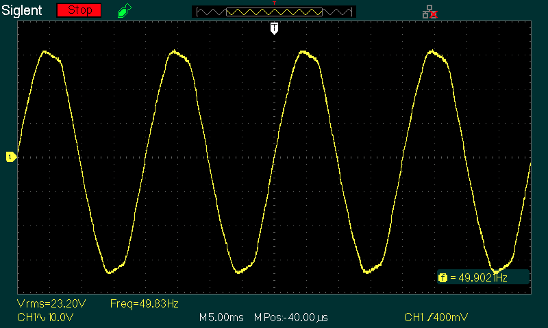
Figure 6 - Mains Waveform At 23V RMS Output
The above is not a sinewave! The first thing to notice is that the peak voltage is not 32.5V as expected (23 × √2), but is only 31V peak. That's because the waveform is distorted, and you can see the 'flat-top' on the peaks. It's not really flat though - it slopes downwards from the initial peak before returning to 'normal'. This is the 'new normal' for mains almost everywhere, regardless of voltage or frequency. The only way to know the actual peak voltage vs. the RMS value is to measure the peak with an oscilloscope, and the RMS voltage with a 'true RMS' reading voltmeter. The 'flat top' is caused by (literally) many thousands of power supplies all drawing current at the peak of the AC waveform, and the supply we are simulating is no different.
Fortunately, it's not imperative that the exact waveform as shown above be provided in a simulation. The important part to get right is a 'flat-top' waveform that approximates the actual, with the right peak and RMS values. Ultimately, it depends on the simulator you use, and how far you are willing to go to get that approximation. If you have a VCVS (voltage controlled voltage source) in the simulator you use, it's quite easy to achieve. The circuit shown below is optimised for 230V mains, but it's easily modified to suit 120V.
Figure 7 - Simulated Flat-Topped Mains Waveform Generator (230V RMS)
There is an additional 'trick' included in the above. The 50Hz generator has a peak output of 330V (233V RMS), and the clipping circuit is perfectly straightforward. It's set up so that the waveform is clipped when it exceeds 315.6V. The RMS voltage is barely affected. As noted above (Figure 2 circuit), the timed switch ensures that the mains is connected at the peak of the AC waveform. Without it, there will be a DC offset in the primary current, and the simulation will have to run for several seconds before the average reaches zero. Real transformers are no different! It takes less time for a 'real' transformer to reach zero DC offset in the primary, largely due to losses and partial unidirectional saturation if the power is applied at the zero crossing. Because the clipped AC waveform is a high impedance, a VCVS (voltage controlled voltage source) was included as a unity gain buffer. This is an 'ideal' part, with an output impedance of zero.
The current waveform is shown next. This is the reason for lower than expected DC voltage, because the current is not a nice continuous flow, but has high amplitude peaks when the diodes conduct. The total power from the mains is 32.52W, with 28.2W dissipated in the load, with the remaining 4.3W dissipated in the transformer (and mains) resistances, as well as the diodes. The filter capacitor dissipates less than 250mW, all due to the ESR.
Figure 8 - Input Voltage & Current Waveform With Flat-Topped Mains Waveform (230V RMS)
With this circuit, the ripple voltage at the output is reduced to 470mV RMS, which is primarily due to the reduced DC output voltage and subsequent reduced current in the load. The capacitor's ripple current is 1.98A, and this is closer to the 'real' value than the other two simulations. In particular, look at the primary current waveform - it's very different from the others shown. Current is supplied to the filter cap and load for a little longer, and the waveshape is modified.
You can verify that this is a good approximation to reality by using one of the ESP current monitors - either Project 139 or Project 139A. These are both very useful tools when working on power supplies, because they let you see the current waveform on a scope, without any risk of contacting live mains.
A very important measurement is the VA rating. In the case shown above, the mains supplies 230V at 240mA, which is 55VA (230V × 240mA). Power factor ( W ÷ VA ) is 0.59, which is typical for most 'linear' power supplies. It's quite obvious that these supplies are not linear, and the term is used to differentiate these supplies from switchmode versions.
When a transformer is followed by a bridge rectifier and filter capacitor, it no longer qualifies as a 'simple load'. The current (primary and secondary) is highly non-linear, and this causes much greater losses than the simple primary and secondary resistance would suggest. This is why transformers are always rated in VA (Volts × Amps), and not watts. VA is equal to watts only if the load is linear (i.e. resistive). Real loads are almost always non-linear, and this affects the regulation of a power supply. Unless you include the primary and secondary resistances in your simulation, the end result will be highly optimistic for the output voltage, and highly pessimistic for filter capacitor ripple current. The inherent series resistance reduces the peak capacitor current, and also reduces output voltage regulation.
The topic is important, and isn't something that's well understood by most hobbyists, although it is generally well understood by engineers. In most cases you'll get a maximum of 75% of the rating in VA as watts of output. This is also known as power factor, and the power factor is determined by dividing output power in watts by VA. 75% is the same as a power factor of 0.75 (unity is the best possible, and can only be achieved with a resistive load on the transformer's secondary).
This is something that's covered in detail in the transformer articles, and power factor is explained in detail in the article Power Factor - The Reality in the 'lamps & energy' section of this website. It's a complex area of electrical theory, but it's important. Most people will assume that one should be able to get 300W (continuous) from a 300VA transformer, but that's only true with a resistive load. In a capacitor-input DC power supply (as shown here), the power (in watts) is around 0.75 of the transformer's VA rating. In reality, this is rarely a limitation, because most power amplifiers draw far less average power than the amp's rated power. Even if driven to the onset of clipping, the average power is typically between 10% to 50% of the amp's rated power.
Note that this is usually not the case with most Class-A amplifiers, and (perhaps surprisingly) guitar amps. The latter are often driven into hard clipping (aka 'overdrive') for extended periods, and using less than a 150VA transformer for a 100W guitar amp would be most unwise. Simulations give you the opportunity to test this for yourself, without risking damage.
While we tend to think that 230V (or 120V) mains will measure the claimed voltage, this tends to happen more by accident than by design. In reality, the mains voltage can vary by ±10%, and sometimes more. This is normal, and designs have to take this into consideration. The claimed supply voltage is 'nominal' (existing in name only), and variations are the rule rather than an exception. The frequency (50 or 60Hz) is also nominal, but is much more tightly controlled because if it were otherwise the supply grid would collapse (and that is not an exaggeration). The mains resistance is added to the transformer's primary resistance, so a transformer with a 4.7 ohm primary should use a series resistor of 5.7 ohms (230V - you can work it out yourself for 120V).
We also need to factor in the resistance of the wiring from the distribution transformer, house wiring and the resistance of the mains lead to our power supply. With 230V mains, this usually works out to be around 1 ohm. I've measured the resistance at 800mΩ, so a 2,300W load (10A) causes a voltage drop of 8V at the wall outlet. In 120V countries, expect this to be roughly ¼ of that with 230V. That means the mains resistance should be about 0.25Ω for 120V mains. That means that around 75-80W is 'lost' just in the mains wiring at maximum current (a current of 10A at 230V or 15A at 120V is assumed). It's very rare for audio equipment to run at maximum power continuously, although many Class-A amplifiers will come close, as will preamps. The latter are not a problem because the current is usually quite low (typically less than ±100mA in most cases).
The typical variation of mains voltage is up to ±10%, so 230V could be anywhere between 207V and 253V. It's usually less, but the variation will always be at least ±5%, a range from 218V to 242V (all RMS). For 120V countries, that gives a range of 108-132V (±10%) or 114-126V (±5%). This needs to be accounted for when designing a power supply, and you also need to remember that the no load (or light load) output voltage from any transformer will always be greater than that at full load (as determined by the regulation figure for the transformer you intend to use).
For example, if the transformer regulation is stated to be 8%, the output voltage will be 8% greater at no load than at full load (resistive load). When used for a DC power supply, the regulation figure is (roughly) double that with a resistive load, as shown above. For our hypothetical 23V, 300VA transformer, the AC output will be 24.8V with no load (giving about 34V DC).
Many low-power supplies will be regulated, most often using a 3-terminal regulator IC such as LM7815/ 7915 or variable regulators such as the LM317 or 337. All regulator ICs require some 'headroom', so the input voltage - including ripple - must be a few volts higher than the output voltage. Should the most negative point on the ripple waveform fall below the minimum necessary, there will be some 'breakthrough' of noise, usually heard as a buzz if it leaks into the audio signal by some means.
For projects like the Project 05 or Project 05-Mini, the suggested secondary voltage is 15V AC, usually with a transformer rated for at least 15VA (500mA secondary current). Because very few preamps will draw anything like that much current, I know that the output voltage will be somewhat higher than claimed, because it's quoted at full load. In general, that means that the DC input will be at least 21V, and usually a bit more. Even if the mains voltage falls by 10%, there's still around 19V before regulation.
The 'dropout' voltage for these regulators varies, but it's usually around 2V. Provided the filter caps are big enough (and the two projects mentioned have plenty of capacitance), even the ripple voltage won't fall low enough to cause problems for typical currents - usually a maximum of around 100mA or so. This is something that must always be considered, but we also have to work with what's available. I would rather specify transformers with an 18V secondary (or two 18V secondaries), but these are difficult to obtain. If ripple breakthrough ever becomes an issue, then it's a simple matter to use 12V regulators instead, with the certain knowledge that all ESP designs will work perfectly happily with ±12V supplies. Many hundreds of preamp regulator boards such as those mentioned have been sold, and no-one has ever had a problem with ripple breakthrough.
That doesn't mean that you don't have to verify your design thoroughly. The final usage has to be considered, as well as available transformer voltages. You need to ensure that you have enough filtering to minimise the ripple. While I have seen regulators similar to those I provide, some people like to skimp on the filter capacitor, with as little as 470µF suggested in some circuits. While it will probably be fine when the mains voltage is at or above the nominal level or with very light loading, ripple breakthrough is almost a certainty at higher current or low mains.
Simulating a power supply is much more complex than most people realise, especially if you want to get as close to the final physical circuit as possible. Mostly, it doesn't matter all that much, because the mains voltage and waveform will be different at different times of day. If your simulation is off by a couple of volts, that's nothing compared to the changes that will occur naturally due to demand on the supply grid. However, it all helps to get a better understanding of what really happens, how much power is lost, and where.
Once you understand the real factors that affect power supplies, you'll have a much better chance of running a simulation that matches the physical version of the circuit. In most cases, the results you get are more than good enough if you use the Figure 4 circuit. Because the mains itself is so variable, there will never be a simulation that is 100% accurate over all conditions unless your simulation is very complex and accommodates all the variables. Because there are so many variables, that would make the simulation overly complex, and this is rarely necessary in practice.
As noted in the introduction, it's extremely difficult to simulate transformer core saturation. Most simulators will include various cores, but almost without exception they are ferrite, suitable only for switchmode supplies. While it might be possible to find a core that works at mains frequencies, I've not been able to find a combination that's usable. The reality is that it doesn't matter, because the transformer models described here will match reality surprisingly well.
There are (of course) countless articles on-line that discuss switchmode power supply (SMPS) simulations, to the extent that the poor old linear supply is almost forgotten. This is a shame, because linear power supplies have traditionally been one of the most reliable DC sources ever used, while most SMPS designs are only guaranteed to work until they don't. The time between 'working' and 'dead' ranges from months to years, vs. decades for linear designs. Yes, linear supplies can (and do) fail, but they are usually easily repaired with no specialised test gear or SMD rework equipment being necessary.
There are no references as such, other than those provided in-line, which are mainly based on articles published by ESP. There are (very) few examples on-line for power supply simulations, but almost nothing I saw could be classified as usable. Some are nothing short of an unmitigated disaster, and manage to get nearly everything wrong. It should come as no real surprise that the main mentions on the Net of anything that follows proper procedures for simulations exists on the ESP website.
There may be some 'scholarly' articles that cover the topic, but these have to be paid for, and are usually expensive. In addition, you don't even know if the material is useful or not until you've paid for it, an unacceptable practice IMO. ESP's policy from the outset has always been that information should be as accurate as possible, and freely available.
The ESP articles referenced are as follows ...
The fourth reference is an article first published by ESP in 2001, and it uses simulations that are almost identical to those shown here. The difference is that it describes the design of linear power supplies, and only makes reference to the simulations. This article shows you how to set up the simulations to get the best results.
The following is not a reference (I only found it when the article was almost complete), but you may find it useful. The simulations shown don't include the timed switch so primary current measurements aren't accurate, but it does provide some good examples that can be modified to suit your application.
Main IndexArticles Index