
|
| Elliott Sound Products | Waveforms & Harmonics |
 Main Index Articles Index Main Index Articles Index |
Most people are aware that a 'perfect' squarewave (50:50 duty-cycle) contains only odd harmonics, with virtually no even harmonics. Less well known is the effect of changing the duty-cycle, which can result in some interesting patterns. This article looks at different duty cycles, and also covers a couple of other waveforms.
This topic isn't covered well elsewhere, and it's actually difficult to get any useful info from the small number of sites that discuss the reliance of a waveshape on its harmonics and vice versa. When the harmonics are changed, so is the waveform - the two are linked and are inseparable. If you change one, you change the other, always.
One other thing needs to be understood with anything that is not a sinewave. 'Ordinary' multimeters will show a voltage, but it's not the RMS value of the waveform. The voltage shown will be highly inaccurate with anything other than a reasonably clean sinewave. For example, with a symmetrical squarewave, a standard multimeter will register an error of +11%. Pulse waveforms can be much worse, and a pulse waveform can be off by -80% or more, depending on the crest factor (determined by the peak value divided by the [true] RMS value). A sinewave has a crest factor of 1.414. This is covered in greater detail in the ESP application note AN-012 - Peak, RMS And Averaging Circuits.
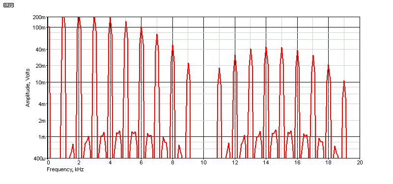
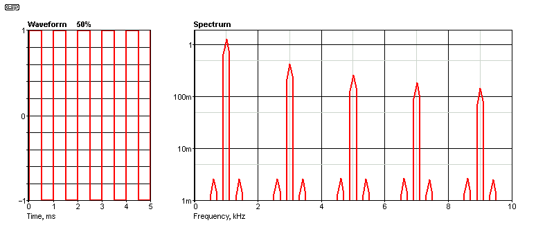
A 'true' squarewave is defined as having a perfect 50:50 duty cycle. This means that the 'on' and 'off' times are identical, not that the waveform looks 'square'. Mostly the appearance is no more than the setting of the vertical axis of the scope used to observe it. When this criterion is satisfied, the harmonic structure is as shown next, with the display extending to 20kHz. In reality, the harmonics extend well beyond that, usually easily reaching into the hundreds of kHz. The ultimate frequency where the harmonics start to fall away quickly is determined by the rise and fall times.
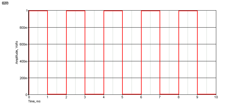
While the figure shows the output from a simulator, there are countless electronic circuits that can generate almost perfect squarewaves, with very fast rise and fall times. The circuitry can be analogue or digital, be unipolar (of one polarity) or truly bipolar. None of these make a difference, but the duty cycle does!
If anyone is interested, the formula for determining the level of any harmonic from a 'true' squarewave is ...
Hn = 4 × A / ( n × π ) Where Hn is the harmonic number and A is the RMS amplitude of the fundamental.
From this, it's easy to work out that with a 1V input, the 3rd harmonic will be at 424mV, the 5th at 255mV and so on. All harmonics are in phase with the fundamental. If there is phase shift involved the 'top' and 'bottom' of the waveform will change, developing ripple or other artefacts.
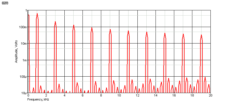
The first (and most important) thing to notice is that there are no even harmonics. For a 1V peak squarewave (500mV RMS), the second harmonic is missing completely, as are all other even harmonics. This gives a squarewave its signature sound, and the relationship between each odd harmonic and its amplitude can be determined mathematically. The same applies to other rectangular waveforms, but the 'true' squarewave is a very common waveform for testing the frequency and transient response of any amplifying circuit.
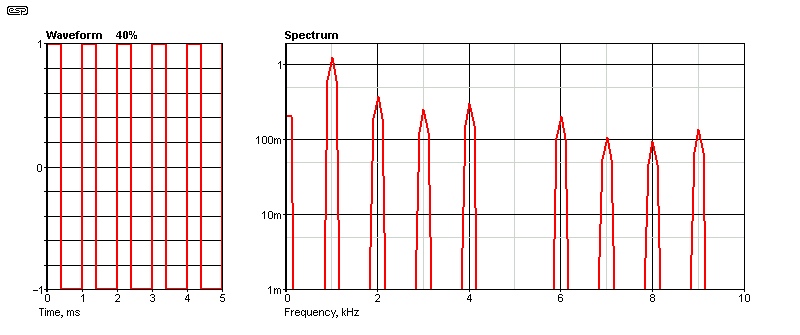
With a perfect 50:50 (aka 50%) duty cycle, even a small variation from the exact ratio will cause vestiges of even harmonics to appear. A great deal depends on the accuracy of the generator used, but the effects are quite audible if you have a generator capable of a variable duty-cycle. Unfortunately, mine will not go beyond 20% (i.e. a 1:4 ratio).
A rectangular wave is any 'square' waveform that doesn't have a 50% duty cycle. This includes (at the limits) pulse waveforms, but these are more commonly referred to as such, and may have a duty cycle of 10% or less. For example, Fig. 2 shows the harmonics of a 33% duty cycle rectangular waveform, in this case 333μs on, and 666μs off. Note that it doesn't matter if the waveform has DC offset (in this case it's from 0 to 1V, with a DC value of 333mV), reverse polarity (0 to -1V) or even inverted (66% on and 33% off). From the harmonics standpoint, nothing changes.
A 33.333:66.666 ratio produces an odd mixture of harmonics, with the 3rd, 6th, 9th, 12th, 15th and 18th harmonics missing entirely (there's no point going beyond 20kHz for audio). So with a 1kHz rectangular wave, you'll get 2kHz, 4kHz, 5kHz, 7kHz, 8Khz and so on. The FFT (Fast Fourier Transform) is shown next.
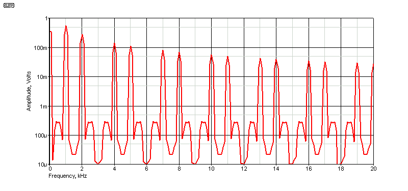
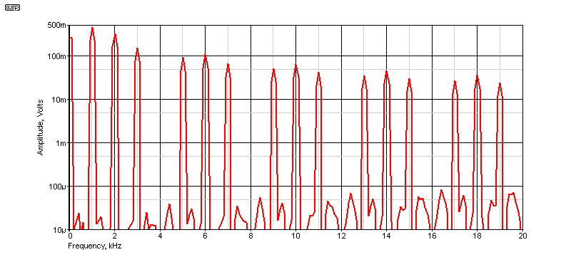
If you use a 25:75 ratio, everything changes again, with the 4th, 8th, 12th and 16th harmonics missing. You should be able to see a pattern emerging - with 50:50 every even harmonic goes away, with 33:66 ratio, every 3rd harmonic in the sequence disappears, and with 25:75 every 4th harmonic in the sequence vanishes. Similar 'disappearances' can be assured with pretty much any ratio, but I've mainly concentrated on 'sensible' figures. A 10% duty cycle will make the 10th harmonic disappear.
The ability to change the harmonic content is used in synthesisers to generate sounds, especially anything that approximates reed instruments. By adding filters and modifying the waveform envelope, a wide selection of different sounds can be created. As the duty cycle is reduced, the amplitude of the harmonics becomes more constant, so with a 1% duty cycle (i.e. 10μs on, 990μs off) the amplitude of the harmonics remains almost constant up to well beyond 20kHz. However, all harmonics are at a low level (about 20mV each from a 1V peak-peak pulse waveform). At 5%, harmonics extend to the 19th, with the 20th missing. Usable levels extend to at least 10kHz.
Using harmonics isn't limited to musical applications. People have been using harmonic tuning with radio frequencies to create frequency doublers and triplers since the early days of radio, and I show an interesting application in the Frequency Changer project, which is designed to change 50Hz to 60Hz (or vice versa) for synchronous clock motors (it can also be used with vinyl turntable motors). This uses either the 5th or 6th harmonic of a pulse waveform to derive a common frequency of 600Hz from the incoming mains.
The different waveforms shown above demonstrate that the harmonics depend on the on-off ratio of the waveform. Sinewaves (ideal ones at least) have no harmonics, so you only get the fundamental frequency, but anything that modifies the waveform (i.e. distortion) causes harmonics to appear.
One very important fact that you must know and be aware of - an asymmetrical waveform has a net DC offset. Any waveform, whether pulse or distorted sine, will develop a net DC value that's determined by the degree of asymmetry. A 1V RMS pulse waveform with 1:2 ratio (e.g. 33.333:66.666) has an average voltage of -333mV DC, and a 25% duty cycle gives a -500mV DC offset. If the voltage is increased to (say) 20V peak, then the DC component becomes much greater (6.6V [33%] or 10V [25%]). As the duty cycle is reduced, the DC value increases. This is one very good reason to never use DC coupling throughout an audio system. Capacitor coupling removes the net DC component, for which your loudspeakers will thank you.
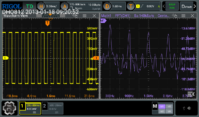
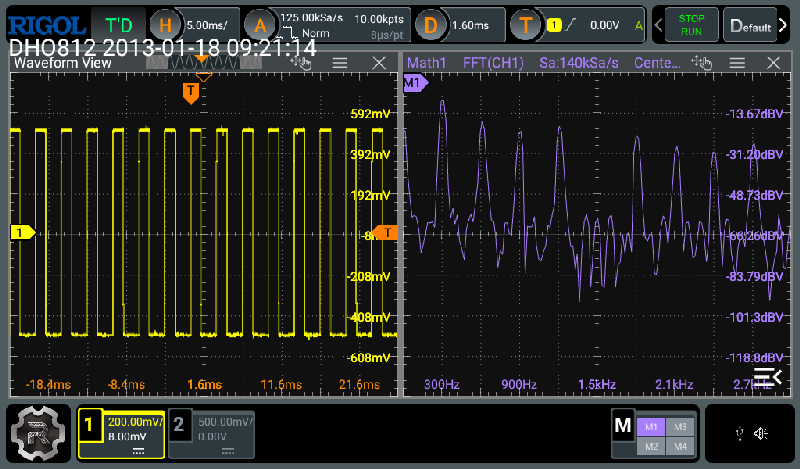
I have some direct captures from my oscilloscope to show the waveform and harmonics of 50%, 40%, 30% and 20% (the minimum duty cycle for my signal generator). Because I didn't use exact ratios, you'll see that the FFTs are different from those simulated, but the trend is quite obvious.
The sound of these is also very different, with the 50% case sounding 'full', and the 20% case sounding 'reedy'. The changing harmonic structure gives a different tone to each sample, although some are not as audible as others. However, they are all different. You can hover your mouse pointer over the following scope captures to see a larger version.
 |  |
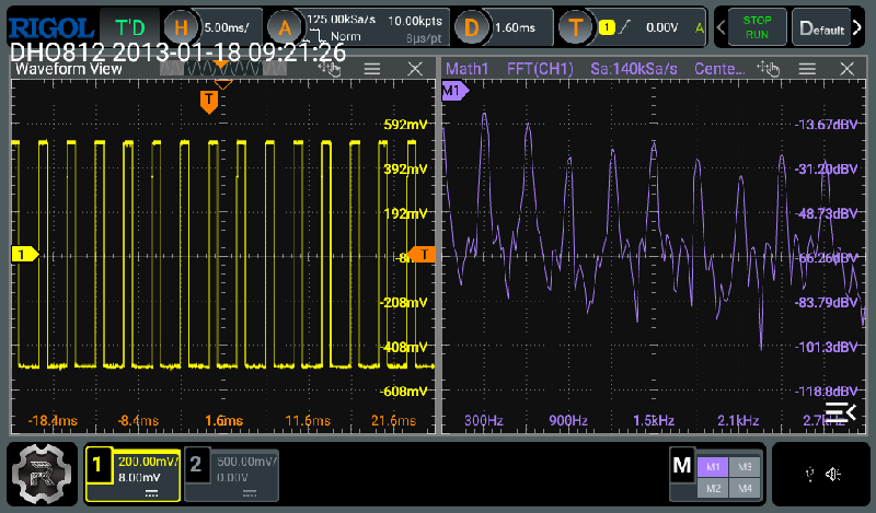 | 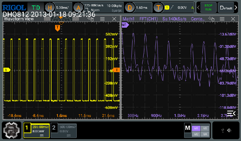 |
The scope captures above show the general trend, but I didn't try to duplicate the simulations exactly. This shows (especially the 30% case) that even a small deviation from the mathematically 'pure' case changes things by far more than you would expect. A simulation of 30% shows the harmonic structure to be identical to the scope capture.
 |  |
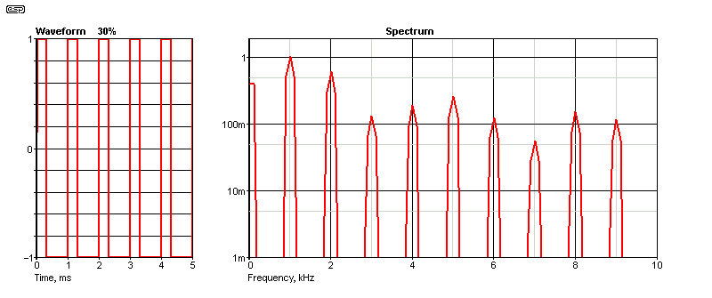 | 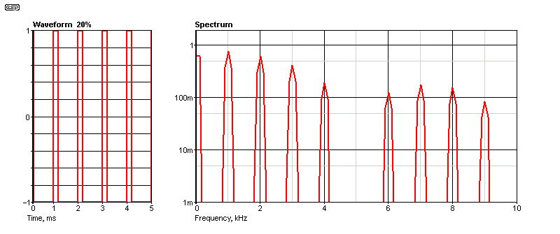 |
The set of images above were taken from the simulator so you can see that the simulation and 'real life' are in agreement. Note that the frequency used was 1kHz, and the spectrum bandwidth for the simulations is 10kHz, arranged so you see roughly the same harmonics as with the oscilloscope. Although the frequency is different (I used 300Hz for the scope captures), the trend is quite clear, and the two show the same progression of harmonics.
The rule with all waveforms is that symmetrical waveforms contain only odd harmonics, while asymmetrical waveforms contain both odd and even harmonics. No common waveform contains only even harmonics. There is one 'exception' to this general rule, and that's a full-wave rectified sinewave. The waveform is asymmetrical, but (for example) with a 1kHz input, the output is 2kHz. The first harmonic is at 4kHz, followed by the 6th, 8th, etc. However, since the fundamental (1kHz) is missing, it's hard to accept that this is a valid waveform for consideration.
A 'sinewave' with only even harmonics can be created by adding harmonics to a fundamental (easy with a simulator or synthesiser, hard to do otherwise), or by including an 'ideal' ½-wave rectifier with resistive summing. The harmonics are all even, and barely a hint of odd harmonics is present. The modified sinewave has just under 26% distortion and it has nothing to recommend it. The waveform was created with the circuit shown next. To create something slightly more realistic (or less unrealistic), the rectified portion of the waveform is attenuated.
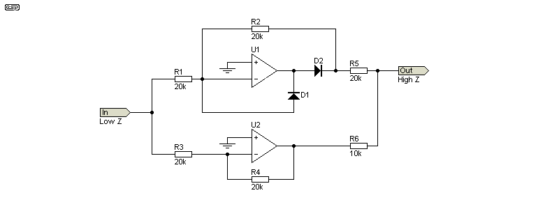
There is no known standard amplifier circuit that can modify a sinewave in the way seen, because it has a form of asymmetry that can't be created with any sensible audio circuit that one can build. I've included it because it's important to understand that even-order only harmonics are very difficult to create, and even if you could, the result would be extremely unsatisfactory. It's been claimed that some JFET circuits can be coaxed into generating only even-order harmonics, but it's not something I've been able to reproduce. I doubt that there will be many people interested in adding a rectifier into their audio circuit, but The Fig. 9 circuit will do the job if that what you think you want (hint - you don't!).
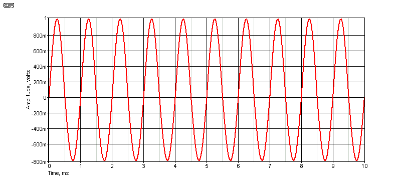
If a sinewave is ½-wave rectified, the harmonics are only even, with the odd harmonics suppressed (by at least 95dB according to the simulator). For example, with a 1V, 1kHz ½-wave rectified sinewave using an ideal precision rectifier (using a simulator and ideal parts), the 'new' 2kHz second harmonic is at 500mV, the 4th harmonic is at 211mV, the 6th at 42mV and so on. If the original (1kHz) signal is added to the rectified output, we get the waveform shown in Fig. 3.2. Bear in mind that a precision rectifier made from real parts will never reach this level of perfection, so it's all rather academic. It goes without saying that music fed through such a circuit will sound utterly revolting. The Fig 3.1 circuit add back some original signal to retain the fundamental.
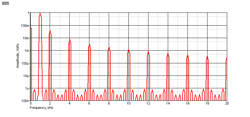
As noted above, a full-wave rectifier does (kind of) generate only even-order harmonics. However, this doesn't really count because it also removes the fundamental! It's also misleading, because the first frequency that's generated is twice the input frequency, so if we use a 1kHz sinewave oscillator and look at the output, we see that the first 'harmonic' is at 2kHz, and those that follow are only even (4kHz, 6kHz, 8kHz, etc.). It's a stretch to consider this to be 'even harmonics only' because the fundamental is removed. There are (of course) websites that claim this is so.
One thing to note is that the spectrum in Fig. 3.3 doesn't look 'quite right'. Everything else we examined has a 'sensible' progression (e.g. fundamental, 2nd harmonic, 3rd harmonic, no 4th harmonic, followed by 5th, 6th, 7th, no 8th, etc.). The harmonics and fundamental form a 'relationship', with everything in tidy little groups of 2 or 3 or 9 (etc.) as shown in earlier plots. This has two at the beginning, then the remaining harmonics are by themselves - the FFT is asymmetrical for frequency.
If we look at 'real' circuits that have asymmetrical distortion, the situation is very different. It doesn't matter if you use a valve (vacuum tube), bipolar transistor, JFET or MOSFET, the distortion products are a predictable mix of odd and even harmonics. You can forget the nonsense you'll hear about valves having 'smooth' or 'nice' even-order harmonics, as this is simply not the case. All simple amplifying devices are nonlinear, including valves.
The other waveforms of interest for music synthesis are the triangle and sawtooth waves. With the latter, I've only covered the case where the return (negative-going) slope is very fast (5μs), but this can be varied. As the slope is increased, fewer upper harmonics are generated and the harmonic content changes (just as it does when the duty cycle of a rectangular wave is varied). For example, if the ramp takes 900μs and the return takes 100μs, the 10th harmonic gets a leave of absence. A more-or-less pure sawtooth waveform is shown next.
As with rectangular waveforms, sawtooth waveforms have a set of harmonics determined by the slope of the two 'faces', so the structure changes from the least distorted (a triangle waveform) to the most (a 'true' sawtooth). Interestingly, an ideal sawtooth waveform produces both odd and even harmonics, despite the fact that it appears to be symmetrical. What we see as symmetrical and what physics determines are quite different. The truly symmetrical 'sawtooth' is, in fact, a triangle.
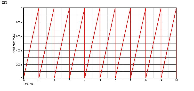
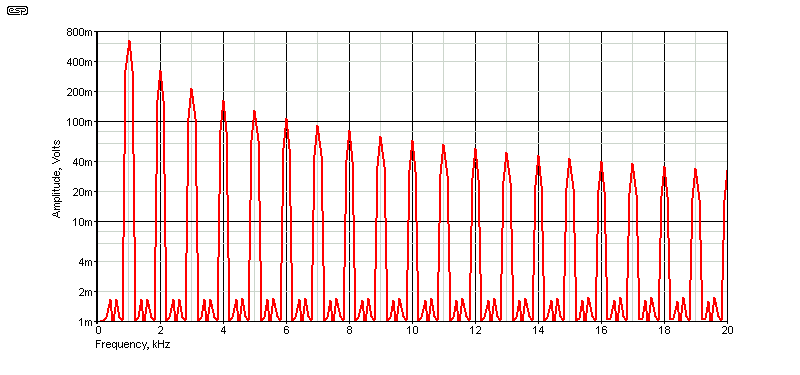
The signal ramps from zero to 1V in 995μs, and returns to zero in 5μs. The harmonic structure is shown next, and you can see that it consists of odd and even harmonics. The level reduction is fairly rapid at first, but remains above 10mV up to 30kHz. This is a very 'rich' tone, well-used in early analogue synthesisers to generate a variety of reed instrument tones.
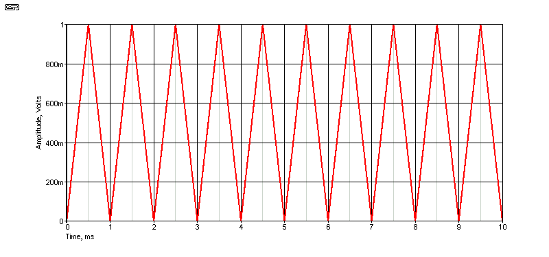
A triangle wave is the fully symmetrical version of a sawtooth. As such, it contains only odd harmonics. Many synthesisers allowed for a sawtooth wave to be adjusted from 'full' sawtooth to triangle. The triangle wave was also used as the input signal for a sinewave converter, which simply rounded the top and bottom of the waveform to approximate a sinewave. The same technique was used in many early signal generators used on many a test bench. The sinewave was never perfect, but it was 'good enough' for most tests, including frequency response. Unlike Wien bridge oscillators (giving a much lower distortion), the synthesised sinewave had zero 'bounce' as the frequency was adjusted. An example of the IC used is the Exar XR2206, a monolithic function generator that provided square, triangle and sinewave outputs.
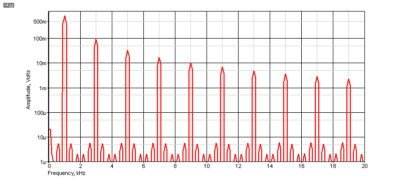
The harmonic structure is shown next. It contains only odd harmonics because the waveform is symmetrical. Even a small deviation from symmetrical (faster rise than fall or vice versa) will introduce even harmonics into the mix, with the amplitudes determined by the degree of asymmetry.
It's worth looking at the process used in early analogue function generators to convert a triangle wave into a 'sinewave'. All that's needed is a very accurate peak amplitude and a pair of matched clipping diodes. These round off the peaks of the waveform, and the amplitude is adjusted for minimum distortion. Devices such as the XR2206 also included a 'symmetry' adjustment to ensure that the triangle wave was as symmetrical as possible. Any asymmetry increases distortion.
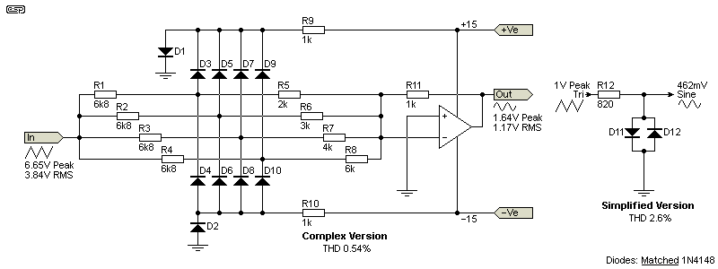
Sinewave shaping can be done with just a pair of diodes, but if you want to get the distortion below 1%, it needs to be more complex. The circuit shown ('Complex Version') does a pretty good job, but the input amplitude has to be tightly controlled. As shown, and with exactly 6.65V peak input, the distortion is about 0.54%, with only odd harmonics present in the output. With a simple 2-diode clipping circuit (also shown in Fig. 4.5) it's difficult to get the distortion below 3%. With an exact 1V peak triangle wave input, matched diodes and a zero ohm source impedance, the 'Simplified Version' manages a distortion of about 2.6%. This is good enough for frequency response testing, but it's not useful for much else.
I haven't shown any waveforms because they aren't at all interesting. The harmonic structure is odd harmonics only for both circuits. Because diodes are used for wave-shaping, these circuits are temperature sensitive, and the output level and distortion will change with the diode temperature. This makes them unsuitable for any precision work, even if the distortion is tolerable for the application. Neither circuit is frequency-sensitive, assuming 'audio' frequencies up to about 100kHz.
Most other waveforms that can be used for synthesis will be a combination of the three main forms; rectangular, triangle or sawtooth. It could be argued that the last two are simply variations on a single theme, but they are (IMO) sufficiently different that we can keep them separate. The only other primary 'waveform' that is used is noise, which can be generated by analogue or digital means. While digital noise is actually quite different from analogue noise, interestingly, they sound virtually identical. Digital noise is generated using what's known as a 'maximum length sequence' (MLS), aka 'pseudo-random binary sequence' (PRBS), aka linear feedback shift register (LFSR). Analogue noise is most often generated by a reverse-biased base-emitter junction using a transistor.
Both types of noise generator are covered on this site, and both can be built using readily available, low-cost, parts. Because analogue noise is analogue, it is more 'real' than a pseudo-random MLS, so it's far less predictable. In theory, a given sample of noise will never be duplicated, but an MLS generator will duplicate the same pattern over and over again. How long it takes for the pattern to be duplicated depends on the length of the sequence - namely how many shift registers are used. For an example of a purely analogue noise generator, see Project 11, and a MLS noise generator is shown in Project 182. The 23-bit MLS noise generator described will run for ~140 seconds with a 60kHz clock before it repeats the sequence. This is long enough to ensure that our auditory memory will usually not detect the repeating pattern. The amplitude of a digital noise source is fairly stable (typically from 0 to 5V), but that changes if you add a filter.
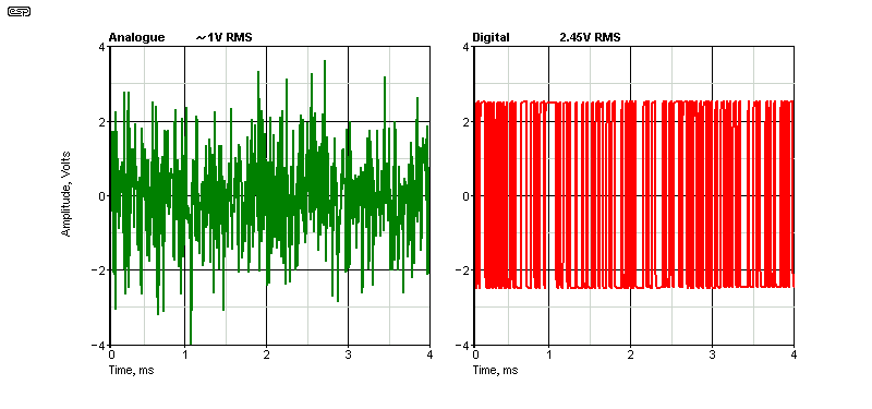
It might not seem possible, but the two waveforms shown above will sound almost identical, and they produce a very similar spectrum (using FFT, and up to ~20kHz). Without filtering, the noise 'colour' is white, having equal power per unit bandwidth. Filtering is used to obtain 'pink' noise, having equal power per octave. Noise is used in waveform synthesis to generate sounds like steam engines, and a small amount of noise can be added to a synthesised flute sound to add realism. It's also used to emulate cymbals and snare drums. By itself, white noise is annoying to listen to because of the excess (to our ears) high-frequency content.
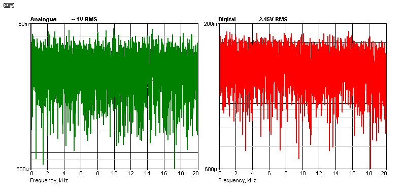
As seen in the above, the general form of the spectrum is almost identical, regardless of whether analogue or digital generation is used. Although the vertical scales are different, this is due to the amplitudes of the two sources being different. With analogue techniques in particular, the noise is so random, that setting a specific level is difficult, as it keeps changing. Pseudo-random (digital) noise may seem more predictable, but it is just as hard to get a constant level. This can be proven by using a bandpass filter and observing that the amplitude is unstable - as it should be!
It's possible to use high-Q tuned filters to obtain 'noisy' notes/ frequencies. In electronics engineering, pink noise is very common because it can be used for frequency response measurements, most commonly using an MLS generator followed by a 3dB/ octave filter. It's possible to filter white noise to get any of the other 'colours', such as brown (not to be confused with the 'brown note'  ). Brown noise is produced by filtering white noise with a 6dB/ octave filter. Brown noise is named after the phenomenon of Brownian Motion (named after Robert Brown - 1773 to 1858), aka 1/f noise. The noise intensity increases with reducing frequencies. It's sometimes called red noise.
All standard filters (as well as non-standard types) can be used on white noise to obtain the type you need for analysis. High-pass, low-pass or band-pass filters will all produce a different outcome. The hardest to get right is for pink noise, as that requires a filter with a 3dB/ octave rolloff (10dB/ decade - decidedly non-standard). Suitable filters (there are two to choose from) are shown in Project 11. This rolloff can only be approximated, because the lowest natural order of any filter is first-order, which has a slope of 6dB/ octave.
There are numerous sites that offer white, pink, brown, grey, and various other 'colours' of noise, many of which are not defined. These are presented as sleep aids, tinnitus masking (tinnitus - constant ringing in the ears [actually the brain, but let's not quibble]) and general relaxation. Some are relaxing, at least at low levels, but some attempts would drive you nuts. Most don't disclose whether the noise was generated using analogue or digital techniques. Ultimately, it doesn't matter, provided that a digital sequence is long enough. 23 bits is pretty good and easily achieved with a few low-cost CMOS ICs.
As this is not a topic that many people have written about, it may be considered by some readers to be 'esoteric'. It's not really, but it is a bit unusual. The only reference is for Brown noise, as all other topics are already covered fairly well throughout the ESP website.
The study of waveforms and their harmonics is interesting (at least I think it is), and most readers will be unaware of the interactions between the exact wave shape and its harmonics. Even seemingly insignificant modifications to the waveform can have unexpected consequences, that can lead people to imagine that something must be wrong. The ability to create a sequence of harmonics with specific frequencies excluded is something that I didn't expect, so I learned something too. The change in timbre is easily demonstrated though, and has been used by synthesiser players since they became popular.
A comment I've made many times on these pages is that with electronics (and audio in general) everything makes a difference. What's important is whether that difference is audible. Few of us listen to specific waveforms for the fun of it, but doing so lets you appreciate how little something needs to change to create an audible change. However, one must be careful not to conflate 'difference' and 'quality', as they are often completely unrelated.
| Main Index Articles Index |