
|
|
| Elliott Sound Products | Compliance Scaling |
 Main Index
Articles Index
Main Index
Articles Index
Since Thiele published his seminal paper on the design of reflex enclosures [ 1 ], his original table of 28 'alignments' has been greatly extended, and these are widely available in both speaker design cook books and on the net.
The impression that seems to be given about these alignments is that they are chiseled in stone, and that if one has a particular driver then one is stuck with the f3 and box volume dictated by the alignment. This however is not true. The fact that the driver's suspension compliance is very insensitive to system parameters, i.e. ...
α, h, f3
means that very many alignments exist that are close to but not quite the 'classical' ones usually published and, as White states, 'virtually any driver can be fitted into an alignment', [ 2, p.892 ]. Thiele states that from certain points of view the suspension compliance is 'unimportant' (his italics), [ 1 , p.188 ].
The miracle of fitting just about any driver to just about any alignment is performed by a procedure called 'compliance scaling', and was, as far as the author is aware first published by Keele, in a 1974 AES paper, [ 3 ].
In addition to compliance scaling two other techniques are outlined, electronically increasing Qt and modifying auxiliary filter damping factor.
Programs available as downloads such as WinISD do a good job of system modeling, the difficulty is that once one strays from the standard alignments that these usually have as defaults, one is in the dark as to what to change and by how much, in order to achieve the desired response.
What follows is a simple method that yields some figures to enter into such programs to give a desired result, and allows you to design a box with a particular driver to achieve a target f3, and or a target box volume, also included is a method of increasing Qt.
But first a word about compliance in relation to the Thiele - Small parameters.
The T-S parameters have become the standard way of specifying the performance parameters of low frequency moving coil drivers. This is because they clump the fundamental physical properties together in such a way as to ease the problem of calculation and specification.
they are related to the physical properties by the following relationships ...
Vas = poC² CmsSd²
Qt = √(Mms / Cms) (1 / Rmt)
Fs = 1 / (2π √(Mms Cms)
Where Cms = suspension compliance (m/N), Mms = moving mass (kg), Sd = diaphragm area (m²), po = density of air (1.2kg / m³), and c = speed of sound (343m/s).
As can be seen compliance plays an important role in all of the above, and also in the system parameters, α, h, f3
As stated by Keele, [ 4 p.254], typical batches of drivers have a 10-20% variation in T-S parameters, and this is largely due to differences in suspension compliance, but luckily for the speaker designer this has little effect upon the frequency response in a given box because of the insensitivity of this to alignment.
The actual scaling procedure entails applying a set of transforms to a 'seed' alignment to give use a new set of system parameters, and this uses a 'normalised compliance' constant, Cn defined as ...
Cms / Cms'
Where Cms is the driver compliance, and Cms' is the driver compliance that would be needed for the driver to be 'correct' for the alignment. Cn then gives us the transform set ...
h = h' √Cn
Qt = Qt' / √Cn
α = α'Cn
f3 / fs = f3' / fs' √Cn
fa = fa' √Cn
Applying these transforms to a standard B4 alignment gives the following results, (Data copied from, [ 2, p.892 ]), for the Cn values of 0.25, 1.0, 4.0 ...
Figure 1 - Transformed B4 Alignments
In the above graph the blue plot is for a Cn = 0.25, this corresponds to a Qt of 0.624, the magenta line is for Cn = 1, Qt = 0.312, the exact B4 alignment, and the green is for a Cn of 4, Qt being 0.156. It can be seen that the greatest deviation is for low Cn values. Figure 2 is for a filter assisted B6 alignment ...
Figure 2 - As Above, With Filter Correction
The Cn values are the same for this plot, and the low Cn plot is somewhat smoother than for the non filter assisted case. Overall the Qt can vary over a wide range without any significant change in overall frequency response and at the low frequencies involved this slight aberration is completely swamped by room effects.
We usually have a specific f3 or box volume in mind when we design a speaker. The techniques that follow allow you to obtain a specific f3 or box volume. Also discussed is the method of alignment adjustment by means of increasing power amplifier source impedance by means of current feedback around the power amplifier, (see Rods article). To make it easier the tables that follow contain two constants, one enables a particular f3 to be obtained, another a particular box size. From the transforms we can write f3 as ...
f3 = (fs / f3' Qt') / (Qt fs')
This separates into two constants, one characteristic of the enclosure, the other of the driver, these are ...
kbf = (f3' qt') / fs' and kdf = fs / Qt
Likewise the expression for Vb ...
Vb = (Vas Qt² Vb') / (Vas Qt'²)
kbv = Vb' / (Vas x Qt'²) and kdv = Vas x Qt²
Table #1 has the values of kbv and kbf for the Qb5 alignments (alignment table in 'Satellites and Subs' article).
| Qt | kbv | kbf | Qt | kbv | kbf | Qt | kbv | kbf | ||
| 0.324 | 4.789 | 0.303 | 0.445 | 9.182 | 0.445 | 0.514 | 7.101 | 0.529 | ||
| 0.318 | 4.702 | 0.318 | 0.425 | 7.372 | 0.490 | 0.517 | 7.099 | 0.533 | ||
| 0.311 | 4.618 | 0.329 | 0.415 | 6.783 | 0.505 | 0.520 | 7.112 | 0.536 | ||
| 0.303 | 4.546 | 0.338 | 0.405 | 6.351 | 0.528 | 0.523 | 7.127 | 0.540 | ||
| 0.295 | 4.464 | 0.345 | 0.394 | 6.009 | 0.541 | 0.526 | 7.157 | 0.543 | ||
| 0.287 | 4.378 | 0.351 | 0.384 | 5.685 | 0.554 | 0.530 | 7.177 | 0.547 | ||
| 0.279 | 4.295 | 0.356 | 0.373 | 5.425 | 0.565 | 0.534 | 7.201 | 0.550 | ||
| 0.271 | 4.217 | 0.361 | 0.362 | 5.202 | 0.575 | 0.538 | 7.258 | 0.554 | ||
| 0.263 | 4.147 | 0.365 | 0.352 | 4.982 | 0.585 | 0.543 | 7.294 | 0.558 | ||
| 0.255 | 4.088 | 0.368 | 0.342 | 4.792 | 0.594 | 0.549 | 7.340 | 0.562 | ||
| 0.247 | 4.041 | 0.370 | 0.331 | 4.659 | 0.599 | 0.555 | 7.412 | 0.566 | ||
| 0.240 | 3.975 | 0.373 | 0.322 | 4.498 | 0.608 | 0.562 | 7.503 | 0.570 | ||
| 0.233 | 3.921 | 0.376 | 0.312 | 4.392 | 0.612 | 0.569 | 7.626 | 0.574 | ||
| 0.226 | 3.880 | 0.378 | 0.303 | 4.280 | 0.618 | 0.577 | 7.781 | 0.577 | ||
| 0.219 | 3.852 | 0.379 | 0.294 | 4.190 | 0.623 | 0.587 | 7.973 | 0.581 | ||
| 0.213 | 3.804 | 0.381 | 0.286 | 4.092 | 0.628 | 0.598 | 8.249 | 0.584 | ||
| 0.207 | 3.767 | 0.383 | 0.278 | 4.013 | 0.632 | 0.610 | 8.614 | 0.587 | ||
| 0.201 | 3.742 | 0.384 | 0.270 | 3.953 | 0.635 | 0.625 | 9.143 | 0.589 | ||
| 0.196 | 3.692 | 0.386 | 0.262 | 3.910 | 0.637 | 0.643 | 9.913 | 0.592 | ||
| 0.190 | 3.692 | 0.386 | 0.255 | 3.851 | 0.640 | 0.664 | 11.228 | 0.594 | ||
| 0.185 | 3.665 | 0.387 | 0.249 | 3.778 | 0.645 | 0.691 | 13.962 | 0.595 |
kdf = 27.4 / 0.281 = fs / Qt = 97.51
This needs ...
kbf = 30 / 97.51 = 0.308
From the QB 5 Class I alignment table the suitable alignment is No. 1 with a kbf = 0.303, so ...
√Cn = 0.324 / 0.281 = 1.153, therefore Cn = 1.329
a = 1.989 x 1.329 = 2.64
h = 0.995 x 1.153 = 1.322
fa = 0.944 x 1.153 = 1.255
multiplying or dividing the a, h and fa data in the QB5 table by Cn or √Cn as appropriate, gives the transformed values ...
Vb = (2 x 81.58) / 2.64 = 61.8 litres
Fb = 27.4 x 1.322 = 36.2 Hz
Fa = 27.4 x 1.255 = 34.4 Hz
Putting these figures into WinISD gives the result ...
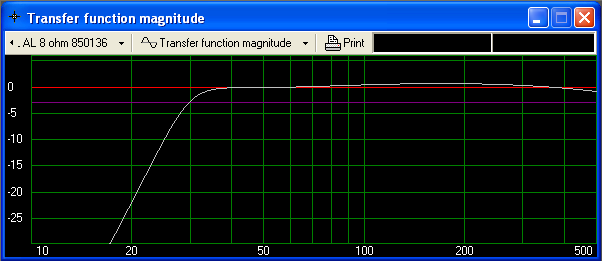
Figure 3 - WinISD Plot of Scaled Peerless Box
By using the compliance scaling and filter assistance this is a much better result than would normally be expected. The filter is a second order high-pass, having a -3dB frequency of 29.8Hz and a Q of 2.141
Should anyone simply select the same driver and run WinISD, the optimum result is actually far from optimal, having a -3dB frequency of almost 47Hz. While the box is smaller, it will be sadly lacking in the bottom end.
Small's power handling parameter 'kp', is a very useful tool in determining the excursion limited power handling of a particular system. I have yet to find any reference to it on the Net except for my QB5 alignment article, I suspect this is because kp is difficult and tedious to calculate, and programs like WinISD provide a plot of maximum SPL. However, I still like to check by calculating kp, and the simplest way I have found is as follows ...
Divide the peak excursion for your transformed alignment by the 'correct' one, and substitute in Small's expression, [ 5, P.439] ...
kp1 = 0.425 / ((f3 / fs)4 j(xmax)2)
Where kp' is the correct 'seed', kp
J(xmax)' = (0.424 / ((f3 / fs)4 / kp)0.5
J(xmax) = ((pkx / pkx') j(max))'
Kp' = 0.425 / ((f3' / fs')4 j(xmax)'2)
In our first example the low peak Excursion is = 1.69mm and the high peak = 0.873mm, an average of 1.28mm. The 'correct' alignment has low peak = 0.532 and high peak = 0.977, averaging 0.755
The correct alignment has a kp of 9.349, giving j(max.)' of 0.131, j(max) is then = 0.222 giving Kp = 5.98
Giving a conservatively rated output of around 105db Peak for a pair before the linear excursion limit is reached, the SLS 213 driver will give more output before excursion limiting, but at the expense of a box twice as large. It should also be noted that since the class I alignments have an average of 6db of boost at around the f3, they need around four times the power that the nominal efficiency would indicate, this is the price we pay for a small box.
We can increase Qt by increasing Qe, and this can be done by increasing the driving amplifiers output impedance by means of current feedback, [ 6 ], (Rods article).
If we write Qe as [ 7 ] ...
Qe = Rvc / Lces ws
We can increase Qe by adding a source resistance to Rvc
Qe' = (Rvc + Ro) / Lces ws
If the Qe we need is = Qe', then The required Qe' is given by ...
Qe' = 1 / (1 / Qt' - 1 / Qm)
Where Qt'= the required Qt. The required source resistance is then ...
Kl = Rvc/Qe
Ro = Qe'Kl - Rvc
[  ] The following diagram shows the essentials of modifying the amplifier's output impedance, giving a circuit that is relatively easily scaled for any loaded gain and a defined output impedance. The calculations for this are fairly straightforward, but only if you can accept an apparently random loaded gain. If you want to specify the loaded gain, the calculations become extremely tedious. While a far better mathematician than the editor may be able to derive a suitable equation, I was unable to do so.
Although I did try this with a spreadsheet (and that's where the formulae I eventually used came from), it is a reiterative process. Those wishing to experiment are encouraged to do so. The formulae shown below work, and the results are an exact science. Calculating the values is anything but, unfortunately.
Essentially, the calculations involve solving for an unbalanced Wheatstone bridge network, with specific desired end results. Of course you can always cheat and use a series resistor of the appropriate value, but this will have to dissipate (and waste) considerable power with any amplifier capable of reasonable output. I can't recommend using a series resistor unless the required output impedance is no more than one ohm.
In essence, the determination of the correct values is not easy. Because we generally need to specify the output impedance, as well as the normal loaded gain (so the amp is in line with others in the system), we end up with too many unknown variables - the circuit may look simple, but calculations for it are not.
Figure 4 - Amplifier With Defined Zout
As can be seen, there is minimal additional complexity to achieve this result, and in my experience the final exact impedance is not overly critical, given the 'real world' variations of a typical loudspeaker driver.
The no-load voltage is 28.5V with an input of 1V, and this drops to 19.2V at 8 ohms, and 14.5V with a 4 ohm load. These voltages are measured across the load, ignoring the voltage drop of the series feedback resistor. Note that a resistive load is assumed, but a speaker has an impedance that varies with frequency.
From this, we can calculate the exact output impedance from ...
I L = VL / RL (where I L = load current, VL = loaded Voltage and RL = load resistance) Z OUT = (VU - VL) / I L (where Z OUT = output impedance, VU = unloaded voltage, VL = loaded voltage) I L = 19.2 / 8 = 2.4 Z OUT = (28.5 - 19.2) / 2.4 = 9.3 / 2.4 = 3.875 Ohms
Note that I have deliberately not developed a single formula to calculate impedance, because no-one will remember it. By showing the basic calculations (using only Ohm's law), it becomes easier to understand the process and remember the method used. An approximate formula to calculate Z OUT is shown below. According to this formula, Z OUT is 3.875 ohms. This is in agreement with the result I obtained above, and with a simulation, and it will be more than acceptable for the normal range of desired impedances. It isn't complex, but it does require either simulation or a bench test to determine the loaded and unloaded voltages. Results will be within a couple of percent of the theoretical value, which is more than good enough when dealing with speakers.
The circuit above is almost identical to that shown in the article / project Variable Amplifier Impedance. By varying R2, R3 and R4, it is possible to achieve a wide range of impedances that will be usable in this application. The circuit can be made variable, however this is not normally useful except for ongoing design and experimentation.
The loudspeaker driver's nominal impedance is used to determine the loaded gain. The preamp is useful because nearly all ESP amps are designed with a gain of 23 (approx. 27dB). However, when you start playing with the output impedance, you'll need a dedicated preamp in front of the power amp, with a gain pot (or trimpot) that lets you adjust the final gain. Mostly, the preamp will only need a gain of about two, and the output is then reduced to get the final gain you need (namely 23 with the nominal impedance).
As shown above, the values apply for the following example. R1 is 22k as used in most ESP amplifier designs, and the feedback resistor (R4) is 0.2 ohm. Using 2.4k (2 x 1.2k in series) for R2 and 1.2k for R3, the output impedance is 3.875 Ohms, and the loaded gain is 16.1 with an 8 ohm load. [ ]
This scheme is especially useful for increasing the Qt of low Qt high efficiency drivers, such as the JBL K140. This driver is still much available on the internet as a re-cone, and is especially designed for bass guitar applications. If we put it into a filter assisted alignment the result is an increase power handling. Increasing Qt has the advantage that the drivers high efficiency is preserved whilst achieving a low enough f3 in a small box. We want f3 = 40Hz for the usual bass guitar tuning.
Looking at the QB5 class I alignments the required f3 / fs of 1.333 is achieved by the alignment No. 7, this needs a Qt of 0.271, and a box of 92 litres ...
Qe' = 1 / (1 / 0.271 - 1 / 5) = 0.287
Ro = 1.68
The above values are perfect, with only the smallest discrepancy which is of no consequence in the final design. WinISD gives the following ..
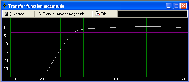
Figure 5 - WinISD Plot of JBL K140 With Modified Qt
This is achieved by using the amplifier set for an output impedance of 1.7 Ohms, and with a second order 40Hz high-pass filter having a Q of 1.658. It is worth noting that using any one or two of the techniques described will not work - the final result is derived only by the combination of compliance scaling, elevated source impedance and filter assistance applied as a complete system solution.
Thiele points out that all other things being equal, doubling Qt results in a +6db peak at the resonant frequency, [ 1 ], i.e.
20 Log(Qt / Qt')
From this we can fit a driver to a particular filter assisted alignment by modifying the fa damping by the amount
dbfa' = dbfa - (20 Log(Qt / Qt'))
With the advent of five and now seven speaker surround systems, there is an increasing need for small speaker systems with good power handling, and the all important SAF index improves with less intrusive enclosures. A typical high quality 150mm. Bass/mid. Driver is the Vifa P17WJ. In this case we fit it to a box that will give an f3 of around 80Hz, making it suitable for use as a satellite, and use a QB5 class II alignment, this optimizes excursion limited power handling.
If we use the QBQ class II alignment No. 14, we have
Vb = 12.6 litres, fb = 68.6 Hz, Fa = 78.1 Hz, 1/Qfa = 1.9
Giving the WinISD plot ...
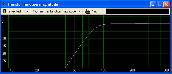
Figure 6 - WinISD Plot of QB5 Alignment Response
In some cases we only want to use a simple passive first order filter, in others we only want to use two passive first order sections, in which case we have a fixed auxiliary filter damping factor of two. This is characteristic of the auxiliary filters in the QB5 class III alignments. In the case of being able to use only a single first order section, the B5 alignments [ 8 ], are useful, these are reproduced in table #2.
| Qt | Vas/vb | Fb/fs | Fa/fs | F3/fs | kbf | kbv |
| 1.320 | 0.0438 | 0.695 | 0.431 | 0.651 | 0.859 | 13.10 |
| 1.230 | 0.0561 | 0.709 | 0.455 | 0.66 | 0.812 | 11.78 |
| 1.120 | 0.0711 | 0.725 | 0.485 | 0.671 | 0.752 | 11.21 |
| 1.010 | 0.0914 | 0.745 | 0.526 | 0.686 | 0.693 | 10.725 |
| 0.881 | 0.126 | 0.774 | 0.588 | 0.712 | 0.627 | 10.225 |
| 0.791 | 0.163 | 0.801 | 0.645 | 0.736 | 0.582 | 9.805 |
| 0.727 | 0.200 | 0.824 | 0.694 | 0.76 | 0.553 | 9.460 |
| 0.666 | 0.251 | 0.852 | 0.746 | 0.79 | 0.526 | 8.920 |
| 0.633 | 0.289 | 0.870 | 0.781 | 0.811 | 0.513 | 8.636 |
| 0.564 | 0.406 | 0.917 | 0.862 | 0.871 | 0.491 | 7.743 |
| 0.529 | 0.499 | 0.948 | 0.917 | 0.915 | 0.484 | 7.161 |
| 0.508 | 0.567 | 0.967 | 0.943 | 0.944 | 0.480 | 6.834 |
| 0.497 | 0.614 | 0.979 | 0.962 | 0.964 | 0.479 | 6.594 |
| 0.489 | 0.645 | 0.987 | 0.98 | 0.977 | 0.478 | 6.484 |
| 0.478 | 0.701 | 1.00 | 1.00 | 1.00 | 0.478 | 6.243 |
| 0.435 | 0.97 | 1.05 | 1.088 | 1.10 | 0.479 | 5.448 |
| 0.392 | 1.39 | 1.10 | 1.20 | 1.25 | 0.490 | 4.682 |
| 0.346 | 2.03 | 1.13 | 1.348 | 1.48 | 0.512 | 4.115 |
| 0.328 | 2.36 | 1.13 | 1.42 | 1.60 | 0.525 | 3.934 |
| 0.317 | 2.55 | 1.13 | 1.466 | 1.68 | 0.533 | 3.902 |
| 0.309 | 2.72 | 1.12 | 1.506 | 1.76 | 0.544 | 3.850 |
| 0.298 | 2.94 | 1.12 | 1.56 | 1.86 | 0.554 | 3.830 |
A driver that is popular for computer speakers is the Tangband, W3-926S. Using a B5 alignment with an F3 = 100Hz gives a box of 4.7 litres, tuned to 105Hz. This achieves its rated xpeak with one Watt of input. If you put this driver into a sealed box the maximum output at 100Hz is 77.9dB, with the B5 box this is raised to 89.9db. Using a QB5 class III box gives a rather large 7.5litres.
It also should be noted that putting a capacitor between 150 and 220µF in series with the driver only changes the frequency response by around 2db. As shown in the Matlab plot of Figure 7 the frequency response with 220µF is not as smooth as with an isolated filter, but is within acceptable limits.
Figure 7 - Capacitor Coupling (Non-Isolated Filter)
In some instances it is convenient to provide one isolated and one non isolated filter, i.e. by means of an input coupling capacitor on the amplifier, and a capacitor in series with the driver. Using a first order isolated filter of twice the non isolated filters f3 gives a plot of Figure 8.
Figure 8 - Isolated Plus Non-Isolated Filter
As illustrated in this article it is possible to fit just about any driver to just about any alignment using the three techniques outlined, or indeed a combination of them.
All efforts have been made to make the calculations of the simple plug in the numbers variety, I apologise where this is not possible. Anybody is at liberty to turn this article into a spread sheet, or some other easy to use form, do not ask me for this however - programming computers is a thing that I dislike, and avoid at all costs (that's the author's comment, not mine).
Main Index
Articles Index